All published articles of this journal are available on ScienceDirect.

Design and Weighting Methods for a Nationally Representative Sample of HIV-infected Adults Receiving Medical Care in the United States-Medical Monitoring Project
Authors Info & Affiliations
Abstract
Background:
Health surveys of the general US population are inadequate for monitoring human immunodeficiency virus (HIV) infection because the relatively low prevalence of the disease (<0.5%) leads to small subpopulation sample sizes.
Objective:
To collect a nationally and locally representative probability sample of HIV-infected adults receiving medical care to monitor clinical and behavioral outcomes, supplementing the data in the National HIV Surveillance System. This paper describes the sample design and weighting methods for the Medical Monitoring Project (MMP) and provides estimates of the size and characteristics of this population.
Methods:
To develop a method for obtaining valid, representative estimates of the in-care population, we implemented a cross-sectional, three-stage design that sampled 23 jurisdictions, then 691 facilities, then 9,344 HIV patients receiving medical care, using probability-proportional-to-size methods. The data weighting process followed standard methods, accounting for the probabilities of selection at each stage and adjusting for nonresponse and multiplicity. Nonresponse adjustments accounted for differing response at both facility and patient levels. Multiplicity adjustments accounted for visits to more than one HIV care facility.
Results:
MMP used a multistage stratified probability sampling design that was approximately self-weighting in each of the 23 project areas and nationally. The probability sample represents the estimated 421,186 HIV-infected adults receiving medical care during January through April 2009. Methods were efficient (i.e., induced small, unequal weighting effects and small standard errors for a range of weighted estimates).
Conclusion:
The information collected through MMP allows monitoring trends in clinical and behavioral outcomes and informs resource allocation for treatment and prevention activities.
INTRODUCTION
Since the emergence of human immunodeficiency virus/acquired immunodeficiency syndrome (HIV/AIDS), the Centers for Disease Control and Prevention (CDC) has expended considerable resources and worked closely with state and local health departments to monitor the epidemic. States passed laws to mandate the reporting of AIDS diagnoses. AIDS reporting started in 1981; by 1986, all 50 states, the District of Columbia, and several US dependent areas had implemented AIDS case reporting [1]. Moreover, all states and many municipalities set up disease surveillance systems to track the number and characteristics of HIV-infected persons. Beginning in 1985, many states implemented HIV case reporting as part of an integrated HIV/AIDS surveillance system. By 2008, all states had implemented confidential, name-based HIV infection reporting [2]. De-identified data on persons with diagnosed HIV infections are sent to CDC for inclusion in the National HIV Surveillance System (NHSS), which measures the burden of HIV disease in the United States, including the number of persons living with HIV, estimated HIV incidence, and transmission rates, stratified by important population characteristics [3].
Following the advent of antiretroviral therapy (ART), deaths due to HIV decreased, and the longevity and general health of persons receiving ART improved [4]. These improvements spurred the desire for more detailed information on the HIV medical care that people were receiving. Because the relatively low prevalence of HIV in the general population (<0.5%) results in small subpopulation sample sizes, general population health surveys are inadequate for this purpose (as would be true for any rare condition). Thus, studies designed to collect data on HIV-infected persons receiving medical care were designed. An early example of such a study was the HIV Cost and Services Utilization Study (HCSUS) [5], which assembled a nationally representative sample of HIV-infected persons receiving regular medical care.
Subsequently, the Institute of Medicine [6] noted the lack of contemporary population-based data and the limitations of previous studies. In response, CDC established the Medical Monitoring Project (MMP). This population-based, supplemental surveillance system was designed to provide nationally representative clinical and behavioral information on HIV-infected adults in care in the United States. Key objectives of MMP include characterizing the population size, experiences, risk behaviors, and clinical outcomes of HIV-infected adults in care for their HIV disease. Accurate information about this population helps guide national, state, and local efforts to allocate resources efficiently and is critical for effective public health action. The evolution, design, and rationale for MMP have been documented in detail [7, 8].
Objectives
In this paper, we review MMP’s sampling procedures, present response rates across project areas, describe the weighting procedures, and provide nationally representative estimates of the size and characteristics of the population of HIV-infected adults in care.
Target Population
The target population for MMP was all HIV-infected adults (18 years and older) in the United States who were receiving medical care for HIV. A comprehensive national list of HIV-infected persons with reported diagnoses is maintained by the NHSS, but that system was not designed to collect in-depth information on behavioral and clinical outcomes. At the time of MMP’s inception, name-based HIV reporting had not been implemented by all states, and the NHSS did not have sufficient identifying information to serve as a sampling frame. Because no comprehensive, up-to-date list of persons in medical care for HIV infection existed nationally at the inception of MMP, devising a strategy to reach this population required a multistage design. Constructing a sampling frame in stages requires vastly less effort than enumerating all patients and makes it feasible to select a nationally representative probability sample [9].
MMP implemented a three-stage sampling design to permit estimation at both the national and local levels.
- Stage 1: A sample was selected from a frame of states and municipalities: primary sampling units (PSUs), referred to collectively as project areas.
- Stage 2: Samples were selected from frames of medical facilities, or groups of medical facilities: secondary sampling units (SSUs) in sampled project areas.
- Stage 3: Patients were selected from frames of selected facilities.
At the project area level, the design was considered a two-stage sampling design (i.e., facilities were the PSUs, and patients were the SSUs). The probability-proportional-to-size (PPS) sampling design allowed for all patients in the area’s MMP target population to be sampled with an equal probability of selection [10, 11].
Data Collection Components
Unlike earlier CDC studies that obtained information on persons in care through either interview or medical record abstraction (MRA) [12, 13], MMP used both of these data collection components, creating a rich, linked data set (Fig. 1). Interviewers administered a 45-minute questionnaire, usually face-to-face or by telephone, on the participant’s health and experiences such as access to medical care, ART treatment and adherence, sexual behavior, drug and alcohol use, HIV prevention activities and counseling, and (for women) gynecologic and reproductive history. MMP was determined by the CDC to be a non-research, public health surveillance activity [14]. Participating states or territories and facilities obtained local institutional review board approval to conduct MMP if required locally [15]. Informed consent was obtained from all interviewed participants.
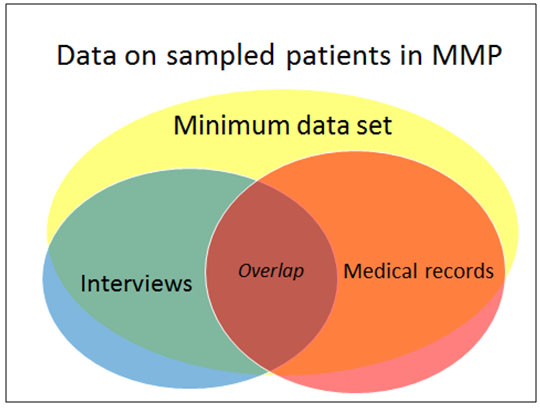
Patient information obtained from MRA included details of prescribed treatment and therapies, comorbidities (such as AIDS-defining opportunistic infections), other conditions, and measures of disease progression (e.g. CD4+ T-lymphocyte cell (CD4) count) and viral suppression (e.g. viral load test results). Additional patient-level data were collected in the minimum data set (MDS), which consisted of demographic variables and other patient-level characteristics extracted from states’ HIV case surveillance registries (Enhanced HIV/AIDS Reporting System [eHARS]) or obtained from HIV care facilities if a case had not yet been reported to the state registry. The MDS contained information for both respondents and nonrespondents and was the basis for nonresponse adjustments. The availability of these data from surveillance registries was a reason for aligning states and PSUs, along with the desire for state-level estimates and the administrative and budgetary convenience of using existing program structures. The main analytic dataset is the “overlap” data set, which includes only persons who have both interview and MRA data [16].
Complementing patient-level information, the facility attributes survey collected data on the characteristics of sampled facilities. This component was the source of information used for nonresponse adjustments at the facility level and to make representative estimates of the characteristics of facilities providing HIV medical care.
METHODS
Overview of MMP Sampling Methods
Probability sampling methods developed and implemented for MMP have been described extensively elsewhere [17] but are outlined here to illustrate how weighting methods align with the sample design.
First-stage Sampling: Project Areas
The first-stage sampling frame consisted of the 50 U.S. states, the District of Columbia, and Puerto Rico. In 2004, 20 areas were selected with PPS (i.e., the measure of size equaled the number of persons reported to be living with a diagnosis of AIDS at the end of 2002).
A number of states had more than a 1/20 share of the size measure and were selected with certainty. Five U.S. cities and 1 county (Chicago, Houston, New York City, Philadelphia, San Francisco, and Los Angeles County) received federal funding for their own local surveillance programs and thus constituted a special circumstance operationally. All six were contained in states that were sampled with certainty, and each became an independent project area, complementary to the rest of the state. Beginning in 2009, budget constraints made it necessary to reduce the number of funded project areas by dropping a random subsample of three moderate-prevalence states. The 23 project areas that participated in the 2009 cycle of MMP (see Table 1) included not only states with high morbidity but also some with moderate and low HIV prevalence, which may not typically be included in a study monitoring HIV care. Each of the US Census divisions (Northeast, South, Midwest, and West) was represented in the sample. Sampling has not been repeated at the PSU level since project inception; thus, the selected states/territories and cities conducting MMP have remained consistent since 2009.
| Project Area | Second-stage Units1 (No.) | Facilities (No.) | Sampled Patients (No.) |
|---|---|---|---|
| California (excluding Los Angeles County and San Francisco) | 30 | 44 | 4442 |
| Chicago | 20 | 27 | 400 |
| Delaware | 15 | 15 | 400 |
| Florida | 30 | 51 | 800 |
| Georgia | 25 | 38 | 400 |
| Houston | 15 | 20 | 400 |
| Illinois (excl. Chicago) | 14 | 34 | 100 |
| Indiana | 10 | 24 | 400 |
| Michigan | 20 | 40 | 400 |
| Mississippi | 10 | 19 | 400 |
| New Jersey | 20 | 25 | 500 |
| Los Angeles County | 20 | 26 | 400 |
| New York City | 25 | 33 | 800 |
| New York State (excl. New York City) | 15 | 33 | 200 |
| North Carolina | 15 | 29 | 400 |
| Oregon | 10 | 21 | 400 |
| Pennsylvania (excl. Philadelphia) | 15 | 25 | 100 |
| Philadelphia | 20 | 26 | 400 |
| Puerto Rico | 15 | 24 | 400 |
| San Francisco | 20 | 28 | 400 |
| Texas (excl. Houston) | 25 | 39 | 400 |
| Virginia | 20 | 29 | 400 |
| Washington | 18 | 41 | 400 |
| TOTAL | 427 | 691 | 9344 |
Second-stage Sampling: Facilities and Second-stage Units
Various sources were used to identify facilities that provide HIV medical care, which were selected at the second stage of sampling [7]. The measure of size used for facility sampling was the estimated number of patients who received care at the facility during January-April of the reference year, the population definition period (PDP). Project areas obtained these estimated patient load (EPL) figures by asking sampled facilities to query their billing databases (ideally) or consult other records to estimate the number of HIV-positive patients seen during the PDP.
Small facilities complicated the PPS sampling design. Below a certain facility size threshold, the patient sampling rate needed to restore equal probability sampling across the two stages of sampling would exceed 100%. To avoid this, small facilities were linked to larger facilities to form groupings whose aggregate measure of size always exceeded this facility size threshold. The facility groupings (which may be thought of as pseudo-clusters) were sampled; that is, all facilities in the linked group were considered to have been sampled if the group was selected. Sampling units are sometimes linked for administrative or logistical reasons, but we linked facilities only to preserve equal probability sampling at the patient sampling stage. Facility samples were selected every 2 years; independent patient samples were selected each year from participating facilities.
Third-stage Sampling: Patients
Information on patient volume obtained from participating sampled facilities was used to determine patient sampling fractions. Although all facilities in the frame were asked for an EPL, the participating facilities provided an actual count of HIV-positive patients aged 18 years and older who received any type of medical care at the facility during the PDP. This updated measure of size, the actual patient load (APL), was used to determine patient sampling probabilities so as to restore equal probabilities of selection across the two stages of sampling. For each sampled facility in a given project area, the product of its selection probability and its patients’ probabilities of selection was constant. The selection probabilities for patients were based on the updated count and were equal for all patients of the same facility, although selection probability differed across facilities.
Sample Sizes and Allocation
Design effects expected for this population under a two-stage clustered design have not been reported. The choice of facility sample size (range: 20-60) was guided by the following considerations. A project area was allocated a slightly larger facility sample size if (1) the area had a large number of facilities, (2) the area had many facilities with few patients, (3) the distribution of the measure of size across facilities was otherwise skewed or irregular, or (4) the state chose to stratify implicitly by geographic region.
The minimum patient sample size per state was set at 400 to ensure sufficient precision [10]. This sample size was not inflated to compensate for patient nonresponse or for the design effect due to clustering. Patient sample sizes were increased for a few project areas (California, Florida, New Jersey, New York City, and Texas), in recognition of the greater burden of HIV/AIDS in those states. Patient sample sizes were reduced for states (Illinois, New York, and Pennsylvania) where the largest urban area bore the greatest burden of HIV/AIDS and was also a participating project area. When the state and the city were combined (Chicago, Illinois; New York City, New York; and Philadelphia, Pennsylvania), sample sizes were adequate for statewide estimates; however, Illinois (excluding Chicago), New York (excluding New York City), and Pennsylvania (excluding Philadelphia) did not have sample sizes large enough to produce independent estimates based on a single year of data.
Patient sample sizes were allocated to participating facilities in accordance with selection probabilities that restored equal probability sampling across the project area. Data on sampled patients were collected in annual, cross-sectional cycles from June of the reference year (the year containing the January-April PDP) through May of the following year. Table 1 indicates the patient sample size for each project area in the 2009 MMP data collection cycle (see Table 1).
Weighting Procedures Used in the 2009 MMP Cycle
Facility-level weights and patient-level weights were computed for each project area and at the national level. Patient-level weights in a project area consisted of a base weight, three nonresponse adjustments, and one multiplicity adjustment [18]. In the next sections, we describe the project area–weights, followed by a discussion of national-level weights as well as state-level weights, which were computed in some instances. We also describe the weight computation for the MRA as well as the overlap data set, which contained individual records with interview and MRA data.
Computation of Base Weights
The patient base weight consists of two components, accounting for the facility’s probability of selection and the patient’s conditional probability of selection given the sampled facility. As some facilities were sampled as part of a group of facilities, or SSUs, the facility base weight (W1) is the inverse of the probability of selection of the SSU,
 |
where P1j is the probability of selection for the SSU in the given project area and j indexes the patient in an SSU.
The second component of the patient base weight is the inverse of the patient’s probability of selection, given that the facility was selected:
 |
where P2j is the probability of selection for patient j in the given sampled facility, or SSU. The design weight is the product of these two base weights.
A series of adjustments was performed on the base weights to reflect nonresponse (including facility, demographic, and survey nonresponse adjustments) and multiplicity. To distinguish these response rate and multiplicity adjustments from the base weights, we use the following notation:
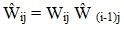 |
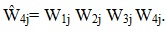
Thus,
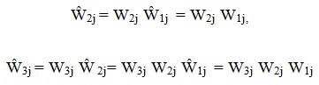 |
and so forth, with the caret indicating the cumulative product of all multiplicative adjustments up to the jth factor.
Response Rate Adjustments
The interview data were subject to the highest levels of nonresponse and therefore potentially subject to greatest nonresponse bias. Response was higher for the other data collection components (i.e., MDS and MRA), which were collected without the requirement of patient consent in areas conducting MMP under their public health authority.
Table 2 presents facility-level and patient-level response rates. Facility participation ranged from 45% to 100% (a rate achieved in five project areas). Adjusted rates of patient-level response ranged from 26% to 71%. The effective combined response rates (facility and patient levels) ranged from 17% to 71%. Adjusted response rates are CASRO rates, standard response rates developed by the Council of American Survey Research Organizations [19]; the denominator includes a term for the estimated number of eligible patients among those whose eligibility status was unknown.
| Project area | Patient counts | Patient rates | Facility participation rate | Combined response rate | ||||||
|---|---|---|---|---|---|---|---|---|---|---|
| Sampled | Eligibility | |||||||||
| Eligible | Ineligible | Unknown | Eligibility | Raw response | Adjusted response | |||||
| Respondent | Nonrespondent | |||||||||
| California (excluding Los Angeles, San Francisco) | 437 | 187 | 67 | 10 | 173 | 0.96 | 0.44 | 0.44 | 0.65 | 0.29 |
| Chicago | 400 | 212 | 64 | 14 | 110 | 0.95 | 0.55 | 0.56 | 0.88 | 0.49 |
| Delaware | 400 | 263 | 135 | 2 | 0 | 1.00 | 0.66 | 0.66 | 1.00 | 0.66 |
| Florida | 781 | 439 | 85 | 53 | 204 | 0.91 | 0.60 | 0.62 | 0.74 | 0.46 |
| Georgia | 357 | 179 | 83 | 12 | 83 | 0.96 | 0.52 | 0.52 | 0.57 | 0.30 |
| Houston | 400 | 163 | 75 | 12 | 150 | 0.95 | 0.42 | 0.43 | 0.68 | 0.29 |
| Illinois (excl. Chicago) | 85 | 43 | 13 | 5 | 24 | 0.92 | 0.54 | 0.55 | 0.45 | 0.25 |
| Indiana | 400 | 237 | 38 | 35 | 90 | 0.89 | 0.65 | 0.67 | 1.00 | 0.67 |
| Los Angeles County | 400 | 249 | 78 | 20 | 53 | 0.94 | 0.66 | 0.66 | 0.80 | 0.53 |
| Michigan | 400 | 165 | 72 | 16 | 147 | 0.94 | 0.43 | 0.44 | 0.62 | 0.27 |
| Mississippi | 400 | 220 | 35 | 26 | 119 | 0.91 | 0.59 | 0.61 | 1.00 | 0.61 |
| New Jersey | 481 | 72 | 24 | 73 | 312 | 0.57 | 0.18 | 0.26 | 0.65 | 0.17 |
| New York City | 740 | 332 | 104 | 57 | 247 | 0.88 | 0.49 | 0.51 | 0.70 | 0.36 |
| New York (excl. New York City) | 187 | 99 | 50 | 9 | 29 | 0.94 | 0.56 | 0.56 | 0.77 | 0.43 |
| North Carolina | 400 | 198 | 60 | 34 | 108 | 0.88 | 0.54 | 0.56 | 0.72 | 0.40 |
| Oregon | 400 | 259 | 79 | 21 | 41 | 0.94 | 0.68 | 0.69 | 1.00 | 0.69 |
| Pennsylvania (excl. Philadelphia) | 91 | 60 | 30 | 0 | 1 | 1.00 | 0.66 | 0.66 | 0.86 | 0.57 |
| Philadelphia | 400 | 260 | 82 | 29 | 29 | 0.92 | 0.70 | 0.71 | 1.00 | 0.71 |
| Puerto Rico | 349 | 211 | 14 | 14 | 110 | 0.94 | 0.63 | 0.64 | 0.83 | 0.54 |
| San Francisco | 400 | 212 | 78 | 19 | 91 | 0.94 | 0.56 | 0.56 | 0.77 | 0.43 |
| Texas (excl. Houston) | 370 | 237 | 60 | 23 | 50 | 0.93 | 0.68 | 0.69 | 0.74 | 0.51 |
| Virginia | 378 | 138 | 71 | 22 | 147 | 0.91 | 0.39 | 0.40 | 0.78 | 0.31 |
| Washington | 382 | 185 | 100 | 19 | 78 | 0.94 | 0.51 | 0.52 | 0.86 | 0.44 |
| Total | 9,038 | 4,620 | 1,497 | 525 | 2,396 | 0.92 | 0.54 | 0.56 | 0.76 | 0.42 |
Note. The number of patients sampled excludes those selected from facilities that presented barriers to participation. A total of 300 patients were sampled from 26 barrier facilities in 2009. Barrier facilities were those in which the project area had no access to any sampled patients; for example, where bureaucratic restrictions barred MMP or facility staff from contacting sampled patients. Patient response rates are adjusted for eligibility.
Nonresponse Adjustment Classes
The purpose of nonresponse adjustments in weighting is to adjust the weights for respondents so that the data better represent both respondents and nonrespondents [20]. The simplest forms of nonresponse adjustments are based on weighting classes defined by using a few selected variables. Ideal weighting classes are homogenous in terms of response rates in each class as well as for the presumed key outcomes. Weighting classes should not have small sample sizes. Specifically, each class needs to contain a sufficient number of respondents not only to permit calculation of meaningful adjustments but also to prevent instability in the adjusted weights. Finally, from a practical perspective, the variables used to define weighting classes must be available both for respondents and nonrespondents. In general, constructing weighting classes by using many variables would violate these statistical guidelines [21].
The most useful data sets for defining weighting classes were the MDS and the facility attributes data set. These data sets had the highest response rates (MDS response rate = 87.8%; facility attributes response rate =100%), provided sufficient number of respondents, and included information on both respondents and nonrespondents to the interview. The menu of nonresponse adjustment variables from these data sets was limited, based on availability of data, to a few key demographics and patient-level characteristics-race, age, and years since diagnosis-as well as facility-level variables such as facility size, type, and affiliation.
The MMP weighting classes defined in different project areas used different weighting class variables. In a project area, and from the subset of key variables available for weighting classes in the MDS and facility attributes data, we analyzed response rates to select the variable(s) most strongly correlated with response propensity for use in constructing appropriate weighting classes, taking care to avoid small cells that might lead to unstable adjustments. Analyses included t tests to compare response rates for subgroups.
Weight Adjustments for Nonresponse
Weight adjustments were conducted at one level for facilities and at two levels for patients.
Facilities were classified as respondents, eligible nonrespondents, or ineligibles. A respondent facility was one that submitted APLs for the PDP or reported that although it was still in business, it had no patients during the PDP. An ineligible facility was one that did not provide outpatient HIV-related medical care to adults.
During the MMP weighting process, several stages of nonresponse adjustments were applied to the patient-level data. Sampled patients were classified into four categories: (1) eligible respondents, (2) eligible nonrespondents, (3) ineligible patients, and (4) patients whose eligibility was unknown. A patient was deemed ineligible for weighting purposes if the patient was younger than 18 years of age at the time of sampling, was not HIV-positive, or did not receive care during the PDP.
Patients were classified as eligible nonrespondents if the interview took place but was not completed, the interview records were missing, or the patients declined to participate. Other patients who did not complete the interview were classified as eligibility unknown.
For many of the patients for whom interview data were unavailable, data were available from the MDS, and facility attributes data were available for all patients from respondent facilities. Therefore, the process consisted of (1) adjusting facility base weights by using facility attributes data, (2) adjusting weights for patients with only MDS data by using attributes data of the facility from which the patient was sampled, and (3) adjusting weights for patients with interview data by using MDS data. These steps are described in the next subsections.
Variables such as facility size, facility type, and patient age, which were significant predictors of participation, were used to create nonresponse adjustment categories. The three nonresponse adjustments for MMP were facility nonresponse adjustments, demographic nonresponse adjustments, and interview nonresponse adjustments. Weighting classes were defined separately for each adjustment and differed by project area.
Facility Nonresponse Adjustment
At the facility level, the definition of weighting classes was limited by the relatively small number of sample facilities in each project area as well as by the limited number of facility-level variables. Moreover, these variables were highly correlated. Therefore, we used facility size to define nonresponse weighting classes in each project area. Two size classes were defined in each project area by using the median EPL for eligible facilities in the project area.
For a particular weighting class, the facility nonresponse adjustment was the ratio of two weighted sums of EPLs: the sum of weights over all eligible facilities-combining both participating facilities (denoted as group A) and nonparticipating facilities (denoted as group B)-divided by the sum of weights over participating facilities only. The weight adjustment (W3) for all facilities in weighting class i is then:
 |
and the base weight for patient j, adjusted for facility non-response, is Ŵ3ij.The weights used in these weighted sums, for both numerator and denominator, were the facility base weights.
Note that the EPL was used because it was available for all facilities in the initial sample, whereas the APL was available only for participating facilities.
Demographic Nonresponse Adjustment
The next adjustment to the patient weights used the MDS to create weighting classes. The MDS was intended to provide demographic information and other, limited patient-level characteristics for the initial sample (respondents and nonrespondents), but the data were not available for all patients in the initial sample because some could not be linked to surveillance registry records. Without patient-level characteristics from MDS or medical records, only less-informative data on facility characteristics could be used for weight adjustments. Thus, when MDS information for respondent patients was missing, we used MRA data as a proxy for the MDS data. Then, for weighting purposes only, we imputed MDS data for the few interview respondents without MDS or MRA values for the key variables used to define weighting classes.
The nonresponse adjustments also used facility-level variables to create project-area–specific weighting classes. We defined binary variables related to responding classes, such as facility size (median, based on APL), university affiliation, and private practice status, which divided the initial patient sample into two approximately equal groups and created groups with differing response rates. Despite many similarities, the factors used for these classes differed by area in this data-driven approach.
The following specifies how we defined the adjustment cells by area:
- Facility size: California, Chicago, Florida, Illinois, New Jersey, Oregon, Texas, and Washington
- Facility’s university affiliation: New York City
- Private practice or public facility: Georgia and San Francisco
- No dichotomized adjustment: Delaware, Houston, Indiana, Los Angeles, Michigan, Mississippi, New York State, North Carolina, Pennsylvania, Philadelphia, Puerto Rico, and Virginia
Within each weighting class, the adjustment factor was the ratio of two sums of weights: (1) the sum of these weights for the entire patient sample and (2) the sum for the patients with MDS data.
The weight adjustment started with the base weights Ŵ3j adjusted for facility nonresponse, as described in the preceding subsection. The adjusted weight for patient j,
 |
is the ratio of two weighted sums. The weighted sum in the denominator is over MDS participants only (class A), and the weighted sum in the numerator is over all MDS sampled patient records (classes A and B). Thus,
 |
Survey Nonresponse Adjustment
At this stage, every sampled patient with MDS data and every nonrespondent had a value for each of the weight components (W1j W2j W3j W4j); hence, for Ŵ4j. The patients without MDS or interview data were then removed from the weighting process, and the respondent sample weights were adjusted so that in each weighting class, the weight sum equaled the sum of the weights for the entire data set (including demographic variables).
For every patient with MDS data in each project area, we identified a categorical variable-a facility characteristic or an MDS variable-that was related to the response rate. As in the preceding step, the variable was chosen on the basis of two conditions-the degree to which it divided the sample of patients with MDS data into two approximately equal groups and the degree to which the response rates of the two groups differed.
The patient nonresponse adjustment cells (or weighting classes) differed by project area. The following specifies how we defined the adjustment cells by area:
- Median facility size: Delaware, Florida, Philadelphia, and San Francisco
- Facility’s university affiliation: Mississippi, Puerto Rico, and Washington
- Private practice or public facility: Chicago, Georgia, Houston, Los Angeles, Michigan, New York City, and North Carolina
- Patient age: Pennsylvania (where the groups were 18-24 years vs. 25 years and older) and Indiana (where the groups were 18-44 years vs. 45 years and older)
- Hispanic/Latino ethnicity: California
- No dichotomized adjustment: Illinois, New Jersey, New York State, Oregon, Texas, and Virginia
For this next adjustment, within each adjustment cell, A was defined as the class of MMP respondents and B as the class of MMP eligible nonrespondents with MDS data (or in some instances, MRA data). We also defined the indicator hj and set hj = 1 if the patient j was eligible, hj = 0 if ineligible; for patients of undetermined eligibility, hj equaled the proportion of eligible patients in the weighting class among patients in the weighting class for whom eligibility was known. The adjustment factor for nonresponse among MDS respondents, W5j, combines the adjusted weights for classes A and B:
 |
Multiplicity Adjustment
After the nonresponse adjustments, a multiplicity adjustment was considered advisable because patients who had received treatment at other eligible facilities during the PDP might have had a higher probability of selection, introducing bias. As in every weight adjustment, the potential for bias reduction needs to be balanced against any increased variability that may be introduced by the adjustment guidelines [21].
Conceptually, patients with a potential for selection from multiple facilities in the frame had a greater probability of selection. The adjustment applied to eligible facilities in the frame whether or not they had been included in the sample.
Multiplicity adjustments typically involve a series of approximations necessary to estimate the multiplicity factor [22]; in terms of MMP, this adjustment used the number of facilities at which the patient received HIV care during the PDP. This adjustment often is expressed in terms of a factor by which the weight is divided. This factor was 1 if the patient visited only one facility during the PDP. The factor equaled 2 if the patient visited a second facility, and more generally, it equaled m if, in total, m eligible facilities were visited during the PDP by the given patient. In the MMP interview, as is common in other data collections, this number was estimated from self-reported data. The multiplicity adjustments we applied in this study did not divide the weights by the factor, but approximated the probability of selection given that the patient could have been selected through more than one facility.
The MMP interview included questions that allowed for approximating the multiplicity factor (m) where the respondent reported the number of other facilities visited for HIV care. Suppose that a patient reported visiting m eligible facilities in the frame. The probability of selection for this patient, considering the probability of not including the patient in the sample, will be the product of not including the patient in any of the m facilities.
The estimated probability of not including the patient may be expressed as:
 |
Thus, the probability of not selecting the patient in any of the m facilities is estimated as:
 |
and the estimated probability of selecting the patient multiple times then becomes:
 |
For weighting purposes, it was assumed that each patient-facility visit would have the same weight, with the same probability of selection for each pair. We estimated
 as the adjusted probability of selecting patient j from any one of the m facilities from which patient j could have been selected. The weight can then be expressed as:
 |
This makes the desired weight adjustment factor:
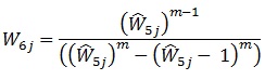 |
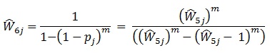
Because relatively few patients went to more than one HIV care facility (7.1% reported going to one additional facility, and only 0.7% reported going to two or more), we imposed a cap of m = 2, which results in the simplified calculation:
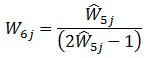 |
Thus, the multiplicity adjusted weight used was:
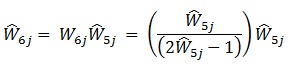 |
Following standard practice, we considered one last step before finalizing project area weights. The intent was to trim weights if any weights in a project area were more than three times the median weight. No project area weights were more than three times the median weight, so no trimming was conducted at this level, and Ŵ6j became the project area weight.
The project area weight was the starting point for the creation of state and national weights, described next.
State and National Weights
The weights described in previous sections applied to the project areas, which are the PSUs of the national sample. In addition to creating project area estimates, we needed to create national estimates and estimates for states in which a city constituted a separate project area from the rest of the state. This subsection describes the computation of weights at the state and the national level.
a. State Weights
For states with separately funded cities, we examined state-level weights for the aggregation of two or three project areas, representing one or two municipalities and the rest of the state, to determine whether an additional adjustment to the weights of the individual constituent areas was needed. Because no weights for the five states with separately funded cities were more than three times their respective median weight in this cycle, we did not need to trim any, and the project area weights (Ŵ6j) became the state weights. Estimates for such a state are based on the aggregation of data across constituent project areas, using the project area weights with no additional adjustment.
b. National Weights
The calculation of national-level weights started with the weights computed for each project area, Ŵ6j. Let W7j be the inverse of the probability of selection of the state from which patient j was sampled. Given that funded cities were in certainty states, W7j was 1.0 for all the patients from any of the cities or the certainty states. The new weight, Ŵ7j, the product of Ŵ6j and W7j, became the initial national weight for patient j.
The final step in producing national weights was weight trimming, implemented to limit the variability in national weights (extreme weights at the national level can lead to large variances, but if one trimmed the extreme weights nationally, the distribution of various demographic characteristics would be distorted). Our solution was to conduct trimming by using weighting categories representing key demographics [23]. This approach divides the sample by demographic characteristics defining weighting categories, in this instance, race/ethnicity (African American, Hispanic/Latino, and other), age (<45 years and ≥45 years), and gender. The median of the Ŵ7j was determined at the national level and for each weighting cell. The weights were capped at three times the smaller of the two medians, and the difference was added proportionately to the patients in the same weighting category.
Let fkj be 1 if patient j is in cell k and 0 otherwise. Let u be the median of Ŵ7j across the nation and uk be the median weight of weighting cell k. Then,
 |
and
 |
constitute the trimmed national weights.
MRA Weights
The MRA weighting procedures were similar to those developed for the interview weights. Also similar were the weight adjustments, including those for nonresponse and multiplicity. However, to control totals, one further adjustment was made at the project area level.
Let WINT be the sum of the interview weights for a given project area. The adjustment factor was then computed as follows, where the sum is over the project area:
 |
Therefore, the adjusted weight is:
 |
These weights add to the same total, WINT, for the project area. Thus Ŵ7j is the MRA weight at the project area level.
We implemented the same procedure at the end for national MRA weights.
Overlaps and Subsets
Weights were created for two subsets of data sets. One was the long form of the interview. The long, or standard, form of the interview was used most of the time. The short form was administered only when the respondent was too ill or otherwise unable to complete the longer standard interview, or when translation was required. A second subset was the overlap, or matched pairs from the interview and MRA data sets. A three-step adjustment process was applied to each data set individually. First, the weights were multiplied by a constant so that their sum equaled the sum of the interview weights for the same project area. Second, the weights were divided by the probability of selection of the project area. Third, the same trimming process was applied to these new weights, using the same procedures and trimming categories as used for the national interview weights.
Variance Estimation
The computation of survey estimates requires the use of appropriate weight and design variables. Taking the survey sampling design into account, we developed strata and cluster variables both at the national and project area levels. Operationally, we ensured that all strata had at least two clusters to provide stratum-level between-cluster variance components.
At the project area level, clusters were defined as linked facilities, or noncertainty SSUs with similar selection probabilities. Strata were created by grouping two or three clusters. The exception was certainty SSUs (certainty facilities), each of which was defined as a stratum. For certainty SSUs within each stratum, patients were the clusters.
At the national level, we first considered certainty strata defined as certainty facilities within certainty project areas. Within certainty project areas, noncertainty SSU units were grouped similarly (i.e., two or three into a stratum). In each such stratum, SSUs were also clusters at the national level. Noncertainty areas were grouped into pairs or triplets to form strata at the national level.
The differing composition of strata and clusters for national and local analyses is an unusual aspect of MMP. Many national, multistage surveys approximate a three-stage design as a two-stage, with-replacement design for variance estimation. The approximation is conservative, meaning that variances are slightly larger than they would be if the complete detail of the sampling scheme were taken into account. Moreover, many software packages used to analyze survey data cannot accommodate more than two stages of sampling when specifying the design. These packages include the less sophisticated SAS procedures (e.g., PROC SURVEYMEANS and PROC SURVEYFREQ) that are used extensively by project area staff for analysis. For local estimates, variance estimation is conditional on the initial sampling of states as PSUs, meaning that this stage of sampling is ignored and that the design is appropriately described as having had only two stages (facilities and patients).
RESULTS
Weighted data from MMP have been analyzed and reported in dozens of peer-reviewed publications. For the present manuscript, we provide estimates for only a few of the many characteristics on which the surveillance system collects data.
Demographic, Behavioral, and Clinical Characteristics of Patients
The sum of weights at the patient level was 421,186. This was the MMP estimate of the size of the population of HIV-infected persons who received medical care in the United States during January-April of 2009. Weighted estimates from the overlap data set further allowed us to characterize this population (Table 3). Most patients were male (71.2%), were non-Hispanic/Latino black (41.4%), and older (39.3% were aged 40-49; 36.2% were aged 50 years and older). Although most were poor (64.4% had an annual household income of less than $20,000), most (81.1%) had insurance coverage, and a slight majority (50.6%) had some college education. A high proportion (88.7%) had been prescribed ART in the past 12 months and 71.6% had achieved viral suppression (the most recent viral load documented was undetectable or less than 200 copies/ml).
| Characteristic | Sample (No.) | Weighted % (Confidence Interval) | CV | Design effect |
|---|---|---|---|---|
| Demographics | ||||
| Age at interview (y) | ||||
| 18-29 | 316 | 7.4 (6.2-8.6) | 0.08 | 2.39 |
| 30-39 | 722 | 17.1 (15.3-18.9) | 0.05 | 2.48 |
| 40-49 | 1647 | 39.3 (37.5-41.1) | 0.02 | 1.54 |
| ≥50 | 1532 | 36.2 (34.3-38.1) | 0.03 | 1.66 |
| Gender | ||||
| Male | 3013 | 71.2 (68.0-74.4) | 0.02 | 5.38 |
| Female | 1139 | 27.2 (24.0-30.4) | 0.06 | 5.47 |
| Transgender | 64 | 1.6 (1.1-2.1) | 0.16 | 1.82 |
| Race/ethnicity | ||||
| Non-Hispanic Black | 1740 | 41.4 (33.3-49.6) | 0.1 | 29.81 |
| Hispanic | 881 | 19.2 (14.2-24.1) | 0.13 | 17.44 |
| Non-Hispanic White | 1395 | 34.6 (28.0-41.1) | 0.1 | 20.50 |
| Other | 199 | 4.8 (3.8-5.9) | 0.11 | 2.43 |
| Foreign born (Country of birth other than US or Puerto Rico) | 529 | 13.1 (11.0-15.2) | 0.08 | 4.33 |
| Sexual and injection drug use behavior | ||||
| Any MSM (MSM only+MSMW) | 1950 | 46.7 (42.0-51.3) | 0.05 | 9.56 |
| MSW only | 1029 | 23.6 (20.9-26.2) | 0.06 | 4.26 |
| Any WSM (WSM only+WSMW) | 1111 | 26.4 (23.3-29.5) | 0.06 | 5.34 |
| Other | 127 | 3.4 (2.5-4.2) | 0.12 | 2.24 |
| Any injection drug use in the past 12 months | 99 | 2.1 (1.2-3.0) | 0.21 | 3.88 |
| Socioeconomicstatus | ||||
| Educational attainment | ||||
| <High School diploma or GED | 985 | 22.6 (20.0-25.1) | 0.06 | 4.03 |
| High school diploma or GED | 1161 | 26.8 (24.1-29.6) | 0.05 | 4.08 |
| Some college or above | 2070 | 50.6 (45.8-55.4) | 0.05 | 9.91 |
| Annual household income (US $) | ||||
| 0-19,999 | 2699 | 64.4 (59.9-69.0) | 0.04 | 9.50 |
| 20,000-39,999 | 690 | 17.7 (15.4-19.9) | 0.07 | 3.75 |
| ≥$40,000 | 691 | 18.0 (14.8-21.1) | 0.09 | 7.11 |
| At or below federal poverty threshold | 1866 | 43.8 (39.6-48.0) | 0.05 | 7.53 |
| Health insurance coverage | ||||
| Health insurance coverage | 3441 | 81.1 (77.3-85.0) | 0.02 | 10.29 |
| Substance use behaviors | ||||
| Current smoker | 1780 | 42.4 (39.7-45.1) | 0.03 | 3.19 |
| Binge drinking (past 30 days) | 720 | 16.4 (15.1-17.8) | 0.04 | 1.45 |
| Noninjection drug use (past 12 months) | 1134 | 27.1 (25.2-28.9) | 0.03 | 1.88 |
| Clinical status and care | ||||
| Time since HIV diagnosis (y) | ||||
| 0-4 | 951 | 23.2 (21.2-25.2) | 0.04 | 2.41 |
| 5-9 | 978 | 23.1 (21.5-24.6) | 0.03 | 1.43 |
| ≥10 | 2283 | 53.8 (51.3-56.3) | 0.02 | 2.75 |
| AIDS (clinical or immunologic diagnosis) | 2897 | 67.6 (65.7-69.6) | 0.01 | 1.86 |
| CD4 lymphocyte count (nadir) | ||||
| 0-199 | 2000 | 46.4 (43.8-48.9) | 0.03 | 2.79 |
| 200-349 | 1112 | 26.9 (25.4-28.3) | 0.03 | 1.17 |
| 350-499 | 586 | 14.5 (13.2-15.8) | 0.05 | 1.48 |
| ≥500 | 485 | 12.3 (10.5-14.0) | 0.07 | 3.10 |
| CD4 lymphocyte count (geometric mean, past 12 months) | ||||
| 0-199 | 543 | 12.4 (11.0-13.9) | 0.06 | 2.01 |
| 200-349 | 743 | 18.5 (17.1-19.8) | 0.04 | 1.29 |
| 350-499 | 1011 | 24.8 (23.4-26.2) | 0.03 | 1.09 |
| ≥500 | 1770 | 44.3 (42.5-46.1) | 0.02 | 1.35 |
| ART (past 12 months) | 3737 | 88.7 (86.9-90.6) | 0.01 | 3.57 |
| Viral suppression: Most recent viral load undetectable or <200 copies/ml | 3016 | 71.6 (68.4-74.9) | 0.02 | 5.60 |
| Sexual risk behavior | ||||
| Any sexual activity | 2640 | 61.8 (59.5-64.2) | 0.02 | 2.49 |
| Sex without a condom | 1032 | 45.3 (40.8-49.9) | 0.05 | 4.86 |
| Sex without a condom with a discordant partner (among persons reporting any condomless sex) | 543 | 52.6 (47.1-58.0) | 0.05 | 3.13 |
Note. Estimates are based on the overlap data set (matched interview and medical record abstraction).
Precision and Efficiency of Estimates
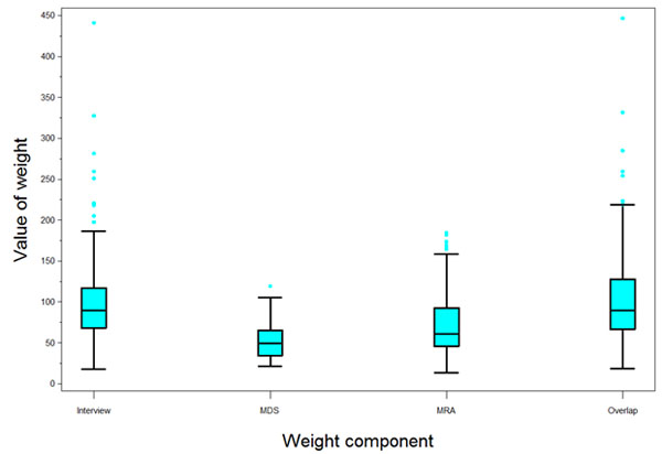
The variability of the 2009 MMP weights was assessed. No reliable external totals were available to gauge any bias components. Table 4 presents the coefficient of variation (CV) of the national weights, as well as the design effect (DEFF) component due to unequal weighting effects. For each data collection component, the design effect due to weighting was 1.3 or less (Table 4). Within project areas, the two-stage probability sampling design was approximately self-weighting. Nonresponse adjustments reflecting different response rates in different groups induced departures from equal weighting and increased the CV of the weights. Across areas, fixed sample sizes and varying population sizes caused further variation in base sampling weights.
| National Weight Type | Sample (No.) | Mean | Standard Deviation |
Minimum | Maximum | Coefficient of Variation |
Design Effect Due to Weighting |
|---|---|---|---|---|---|---|---|
| MDS | 8202 | 51.4 | 18.1 | 21.4 | 119.3 | 35.3 | 1.1 |
| Interview weight | 4415 | 95.4 | 44.1 | 17.6 | 441.3 | 46.2 | 1.2 |
| MRA | 5657 | 74.5 | 41.7 | 13.6 | 184.7 | 56.0 | 1.3 |
| Overlap | 4217 | 99.9 | 48.0 | 18.2 | 446.9 | 48.0 | 1.2 |
The relative standard error-computed as the standard error divided by the estimate itself-did not exceed 10% for weighted estimates of important variables as estimated by using SAS PROC SURVEYMEANS. However, the DEFF was very large for race/ethnicity and for variables likely to be associated with race (Table 3). The large DEFFs were due to clustering effects rather than unequal weighting effects, which were small (Table 4). Large clustering effects resulted when patients within a facility or within a project area had similar characteristics (notably, race/ethnicity).
As the level of nonresponse increased across data sets, so did the average magnitude of each of the weight variables as well as the spread (Fig. 2).
DISCUSSION
Since HCSUS, which collected data from January 1997 through December 1998, no nationally representative estimates have been available for HIV-infected persons receiving medical care in the United States. HCSUS did not produce representative estimates at the state or metropolitan level, but those estimates can now be produced for MMP project areas that were operationally successful and achieved adequate response rates.
In both public opinion and public health research, sample surveys in general have found it difficult in recent years to achieve high response rates. The Behavioral Risk Factor Surveillance System (BRFSS), a national and state-level telephone survey of the general US population, after low response rates in recent years, has changed its sampling and weighting methods to compensate. In 2009, BRFSS response rates for states ranged from 37.9% to 66.9% (median, 52.5%) [24]. In comparison, in 2009, MMP combined response rates for project areas ranged from 17.2% to 70.5% (median, 44.3%). This combined rate, the unweighted product of the facility-level and patient-level rates, reflects the cumulative effect of nonresponse across both stages of sampling. Examining its components, however, MMP patient-level response rates compared favorably with BRFSS response rates, ranging from 26.4% to 70.5% (median, 56.3%). MMP facility-level response rates (median, 77.4%) compared favorably with the average response rate of 60.6% achieved by the National Ambulatory Medical Care Survey (a three-stage design similar to that of MMP) in its second stage of sampling during 2005-2010 [25]. Surveys that use a named list for sampling often achieve higher response rates than those that choose respondents randomly (e.g., random-digit dialing surveys or household surveys) because they are able to personalize contact efforts and appeals to participate [26]. Lower response rates are, however, common for surveys of stigmatized or minority populations [27]. Although the overall MMP response rates were not as high as desired, they were not appreciably lower than those for many other national health surveys whose results are widely used. And although a high nonresponse rate is not in itself an indication of nonresponse bias [28], research is under way to look at the quality of MMP estimates for important indicators of nonresponse and for demographic subgroups.
The very large DEFF for estimates by race/ethnicity is due to clustering effects rather than unequal weighting effects (the design effect due to weighting affects all estimates of characteristics equally, yet few have large DEFFs). The effect is striking for national estimates but is still large for local estimates. The racial and ethnic composition of U.S. states and cities differs greatly, and the same is true of the patient mix of facilities in states and cities. This disadvantage of larger standard errors for some estimates is offset by the convenience of constructing a sampling frame in stages. A large number of geographically dispersed clusters, with the associated burden of recruiting and managing more sites, could become unmanageable. For similar reasons, large DEFFs are common in other multistage surveys with geographic clustering or homogeneity of subjects within clusters. For example, in estimating demographic characteristics of the U.S. population by using public-use data from the National Health and Nutrition Examination Survey (2007-2008) or the National Health Interview Survey (2009), DEFFs were much larger for estimates by race/ethnicity than for estimates by gender, age, or education. Many of the characteristics that MMP measures are influenced greatly by provider practices, which may be similar for most patients of the same provider. Larger standard errors make it more difficult to detect significant differences by race and ethnicity, an area of great concern for CDC and public health in general. Despite the large DEFF for race, however, standard errors for estimated characteristics by race are moderate, and the 4.9 percentage point difference in the prevalence of receipt of ART among white (92.6%; 95% CI = (91.4-93.7)) and black patients in care (87.7%; 95% CI = (86.1-89.3)) was significant in the 2009 national data. It is possible to detect differences in prevalence of 5% or even less for other outcomes and for covariates that have smaller DEFFs and standard errors, but except for rare outcomes, such small differences for these characteristics are unlikely to be of practical (as opposed to statistical) significance.
The 2009 MMP weighting methods described in this manuscript induce small, unequal weighting effects and small standard errors for a range of weighted estimates. Having learned much from the first time through the entire weighting process, we made several refinements for the 2010 MMP cycle. These modifications, discussed elsewhere [29], allowed the integrated weighting of all data sets at the same time. Design variables were also modified in the 2010 MMP cycle. Among several advantages, a common set of design variables and an improved numbering scheme for designating strata and clusters can support variance estimation for all data sets. For the 2011 cycle, moreover, we implemented an enhanced nonresponse analysis as part of the weighting process.
We have also modified our facility sampling method for the 2013 data collection cycle and beyond. We moved to a stratified design, forming strata for the largest (certainty selections), medium-sized, and small facilities, still using estimated patient volumes, but without linking facilities into clusters. This change to disproportionate sampling increased the variance of population estimates slightly, but it led to the selection of fewer small facilities, which improved response rates and increased project efficiency. It also simplified the sampling and weighting procedures.
CONCLUSION
MMP used a multistage stratified probability sampling design that is approximately self-weighting in each of the 23 project areas. The weighting process accounted for the probabilities of selection at each stage and adjusted for nonresponse and multiplicity. Nonresponse adjustments accounted for the differing response rates at the facility and patient levels in project areas. Multiplicity adjustments, although their magnitude was small, accounted for the potential visits to several facilities that patients may have made during the PDP.
The MMP surveillance system provides annual estimates for the HIV-infected adult population in the United States. Because MMP is an ongoing supplemental surveillance system, the information collected will allow us to monitor trends in clinical and behavioral outcomes and can inform resource allocation for treatment and prevention activities in the United States. MMP methods could be adapted to monitor lower-prevalence populations of interest or to evaluate outcomes and clinical care for other rare conditions.
CONFLICT OF INTEREST
The authors confirm that this article content has no conflict of interest.
ACKNOWLEDGEMENTS
Funding for the Medical Monitoring Project is provided by a cooperative agreement (PS09-937) from the Centers for Disease Control and Prevention.
DISCLAIMER
The findings and conclusions in this report are those of the authors and do not necessarily represent the official position of the Centers for Disease Control and Prevention.